Assuming that you have Gaussian distributed errors between the input and output points, and assuming that the errors are additive, you can solve this by classic least squares. It boils down to having an overdetermined linear system of equations where each constraint defines one input-output observation. Solving this overdetermined linear system with the least amount of residual error is the solution you're looking for.
Caveat
Jubobs made a very interesting point in his comment to me below. The parameters that minimize this residual error don't, in general, minimize the residual error of the original problem. This linearization step allows us to solve the parameters in an easier way, but it isn't the equivalent problem. However, it is usually accepted in practice as the solution is good enough.
To get this into a linear system, we need to do some clever rearranging. Because you want to fit a series of points using an exponential model, the relationship between the input x and output y is:

To get this to be "linear", we can take the natural logarithm of both sides:

By using the fact that ln(ab) = ln(a) + ln(b), we have:

Also knowing that  , this simplifies to:

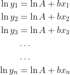
As you can see, the above equation is now "linear" with respect to log-space. Given a bunch of x and y values, so (x_1, x_2, ..., x_n) and (y_1, y_2, ..., y_n), we can concatenate a bunch of equations together in a linear system:

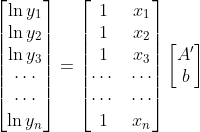
If we let ln(A) = A' for ease of notation, and rearranging this so that it's in matrix form, we get:

Therefore, we simply need to solve for A' and b, and you can do that by the pseudoinverse. Specifically, the above problem is of the form:

Therefore, we need to solve for X, and so:

M^{+} is the pseudoinverse of the matrix. Once you're done, simply take the exp operator on A' to get the original A. MATLAB has very efficient linear system solvers and least-squares solvers. Specifically, you can use the ldivide operator. All you have to do is create the M matrix from the x values, create a vector of y values and solve your system. It's really simply:
x = ...; %// Define numbers here - either row or column vectors
y = ...;
M = [ones(numel(x),1), x(:)]; %// Ensure x is a column vector
lny = log(y(:)); %// Ensure y is a column vector and take ln

X = M  lny; %// Solve for parameters
A = exp(X(1)); %// Solve for A
b = X(2); %// Get b
Therefore, using your x and y values, this is what I get:
A =

    1.3882

b =

   -11.508
If we plot the above points as well as an exponential curve that fits the line, we can do:
xval = linspace(min(x), max(x));
yval = A*exp(b*xval);
plot(x,y,'r.',xval,yval,'b');
The first line of code defines a bunch of x values that span between the smallest and largest x value for our data set. For the next line, we then take the x values and run them through our exponential model. Finally, we plot both the original data points, as well as the exponential curve with the parameters found through the above procedure together. The points are in red while the line is in blue.
We get:

I think that looks pretty good! For those people who have noticed, the above plot looks a bit different than a normal plot and figure window that is produced by MATLAB. That plot was generated in Octave as I don't have MATLAB on the computer that I'm currently working on. However, the above code should still work in MATLAB.
